
Artificial Intelligence Beginnings
Build a Neural Network from scratch in Python
Objective
This post will explain how to create a Neural Network from scratch, using just the Python language, and how to use it to examine cars and predict their mileage per gallon.
First, there are some concepts that should be explained:
The Network
A Neural Network is one of the most commonly used computational models to apply Artificial Intelligence to real-world problems. It consists of sets of units, called neurons, connected to each other to transmit and process signals.
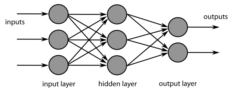
Image by H3llkn0wz / CC BY-SA 3.0
Each neuron is connected to others by links. Through them, they receive information, evaluate it, and spread the outcome of that evaluation, which can be either a signal to highlight a feature or to attenuate it.
The network also has one ore more Final Neurons that will take signals from previous ones and will produce that can be a real number (for regression problems) or a set of values (for classification problems).
Structure
Commonly, Neural Networks are implemented in the form of several neuron layers. The first layer, called the input layer or layer 0, represents the different object features that are evaluated. It differentiates from all the other layers as it doesn’t perform any calculations, just represents the data fed to the network.
In our example, the first layer will hold the features of the cars that will be examined. For example the number of cylinders, weight, acceleration, year and manufacturing origin, etc.
Then, the model will contain two hidden layers. They are called hidden because they don’t connect directly to the inputs or outputs. They will be responsible for evaluating the relationship between the different characteristics from the previous layer and issuing a result to the next layer.
Finally, we will have an output layer, which will obtain the last hidden layer results and will calculate the distance that the car can travel with a gallon of fuel.
The following image is an example of the connections between the neurons of the different layers:
Copyright 2021 Tensorflow: Usage authorized under Apache License 2.0
Neurons
Each layer will be formed by several neurons, except the last layer, the output layer, which in this example will have only one neuron for our problem.
Each of the network’s neurons will be represented by the following formula:
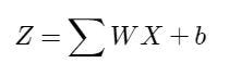
Image by author
Where X is a vector (one-dimensional matrix) with the information coming from the neurons of the previous layer. In the case of the first hidden layer, it will just receive the features of the car from the input layer.
W is a vector that will assign a weight at each value from the neurons of the previous layer. They are one of the main components that will be optimized for the network to produce real results.
b is a value that will apply an offset (BIAS) to the result and will also be optimized.
Image from: www.MLinGIFS.aqeel-anwar.com Author: Aqeel Anwar Usage authorized
Non-linear Activation
The latter function is a linear one. If all the neurons were linear functions, the result of the neural network would also be another linear function. This would not allow the network to identify complex relationships that exist between the features.
To solve this, a non-linear component is added to each neuron, called the activation function. In our case, we will use a commonly used activation function called ReLU (from Rectified Linear Unit), which is nothing more than:
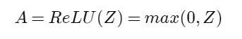
Image by author
So the complete formula of each neuron, except for that of the output layer, will be:
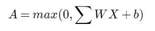
Image by author
Final Linear Activation
As the goal is to predict a value (regression), instead of detecting or classifying an object (classification), the neuron of the output layer, must generate a real value. So it will not have a non-linear activation applied.
The formula of this neuron will be just:
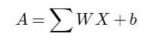
Image by author
Optimization of the Neural Network: aka Learning
The network learning process will involve searching values for the weights W and offsets b that when you feed the network with the data of a car, it will produce the result we want to estimate: the mileage per gallon of that car.
Logic:
To find the W and b values, first, we initialize them with:
- W: Random values that follow a normal distribution * 0.01
- b: Just with 0
Then, repeat the following steps several times (we will call each iteration of this loop an Epoch):
- Feed the network with the characteristics of a car or several cars (in case our network is capable of processing several input data in parallel).
- Perform the calculations of the neuronal network (called forward propagation), multiplying the weights by the input values, adding the offsets, and applying the activation functions layer by layer, until we get the final value.
- Calculate the error (or difference) between the estimated value of the network and the car real value which we will call J(W, b) and will represent the Mean Squared Error in our example.
- From the back to the beginning (a process called backward propagation), using the difference obtained, we will calculate the derivatives for the weights W and the offset b using the following formulas:
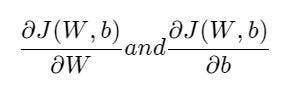
Image by author
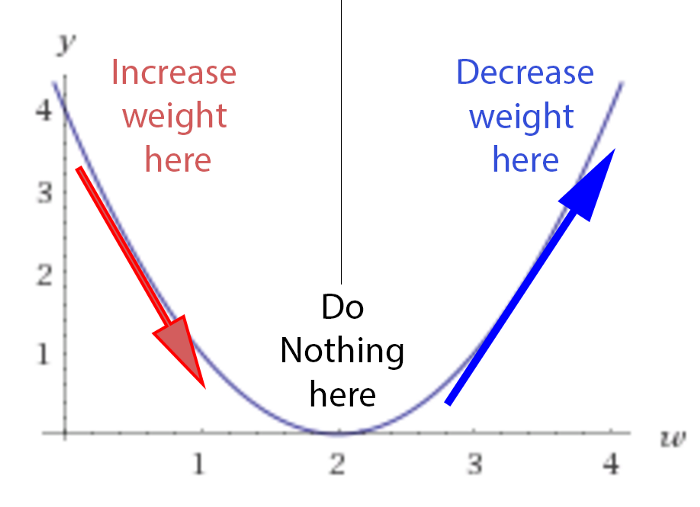
5. With the derivatives, we proceed to modify the weights to bring them closer to the point where the difference reaches a minimum. For this, we multiply the derivative by an α value (called Learning Rate) and we will subtract it to the corresponding weights:
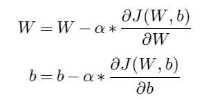
Image by author
6. With the updated weights, we repeat all the previous steps until the error, the difference between the predictions of the network and the actual values, is acceptably small.
The Code
In practice, the optimization of the neural network is not performed one example at a time. There are code libraries that use the capabilities of the modern CPU, GPU, and TPU to perform calculations simultaneously on many examples.
In our case, we will use the Python language and the Numpy library to perform the calculations on all examples simultaneously and obtain a better performance.
The Model
We will define the structure (number of neurons in the first and second hidden layers) and create the model of our Neural Network:
The forward propagation function
It computes the network predictions
The cost function
It measures the difference between the network estimation and the real values:
The backward propagation function
It calculates the derivatives of the network functions
The update weights function
It allows our network to get closer to the expected result
The Data
With the model defined, now we will train the Neural Network with the classic Auto MPG dataset to predict the fuel efficiency of the late-1970s and early 1980s automobiles. The dataset provides a description of many automobiles from that time period. This description includes attributes like cylinders, displacement, horsepower, and weight.
It’s not the objective of this article to go into detail on how to pre-process the data to be fed in the Network. We will just say that the dataset is normalized and split in two, a training set used for the network optimization and a test set used to validate the trained network:
And finally, the code to create and train the network, and evaluate its predictions:
After training the Network finishes, we use it to predict the MPG for the cars in the test set and compare them with their real MPG values.
The predictions are not perfect but near the real MPG values.
Predictions: 29, 26, 30, 32, 25, 28, 42, 34, 29, 28
Real Values: 26, 22, 32, 36, 27, 27, 44, 32, 28, 31
Run the example yourself
To see how this example performs, you can open this Google Colaboratory Notebook, and directly run it in your browser.
Conclusions
This was a simplified regression problem, addressed with a Neural Network written in Python, that presents the very basic but fundamental working concepts of all networks.
There were a lot of omitted concepts on purpose in this example as they may frighten some people. In a real-world project, they will need to be considered. Some of them are:
- The data availability, cleanness, balance between classes, distribution, and how to process it.
- The different network models for different problems (like the one presented for regression and classification tasks, Convolutional networks for Image detection, Recurrent network for sequential series (language translation, stock market forecasting), etc.).
- Different optimization methods (batch Gradient Descent like in this model, mini-batch G.D., Momentum, RMSProp, Adam, etc), and hyperparameter optimizations (layer quantity and size, learning rate, momentum parameters, activation and cost functions used).
- Common problems and how to solve them (Bias and Variance, Exploding or Diminishing gradients, Regularization, Dropout, etc).
- Specialized Hardware for computation speed up (like CPU SIMD instructions, GPUs and TPUs).
We hope that having seen that it is possible to start with a really simple implementation, without needing specialized libraries or hardware, will increase your interest in the exciting field of Artificial Intelligence.
To learn more about this field, two of the common starting point are the Deep Learning and Neural Network book from Michael Nielsen and the Deep Learning book from Ian Goodfellow.
And, If you have some interest in the visual arts, this article about Artistic Style transfer using AI might also be worth reading.